Out Of This World Tips About How To Build Charts In Excel
Excel Quick And Simple Charts Tutorial - Youtube
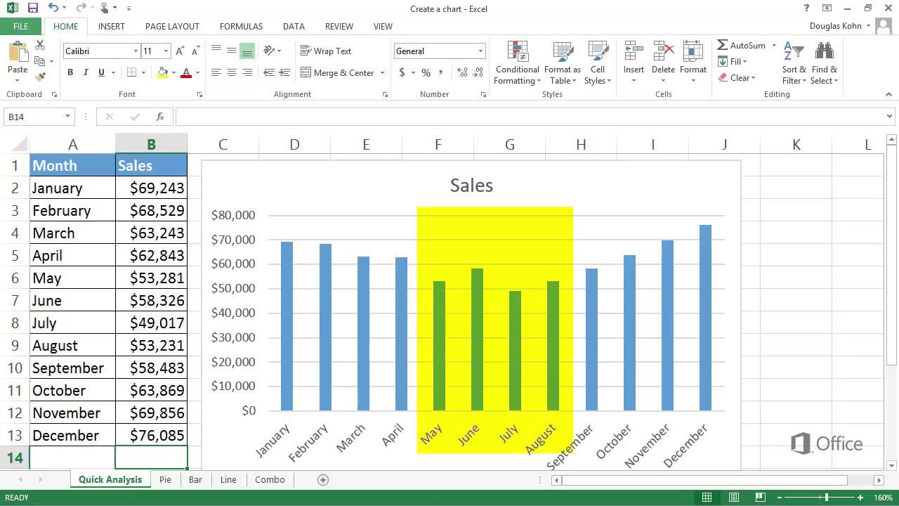
Video: Create A Chart
How To Create A Chart In Excel From Multiple Sheets
How To Create Charts In Excel (in Easy Steps)
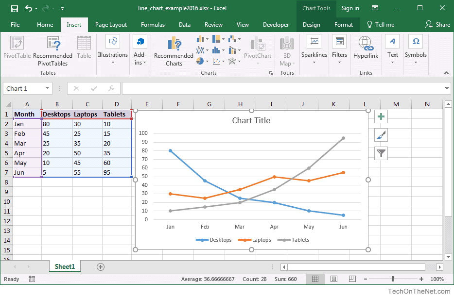
Ms Excel 2016: How To Create A Line Chart
How To Make A Chart Or Graph In Excel | Customguide

You now have your simple run chart as a result:
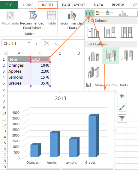
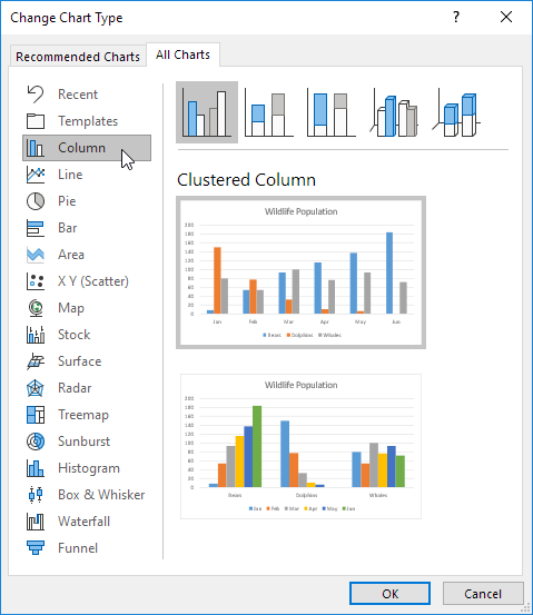
How to build charts in excel. Now, use your named ranges to create the chart. On the insert tab, in the charts group, click the. Finally, select a 2d bar chart from.
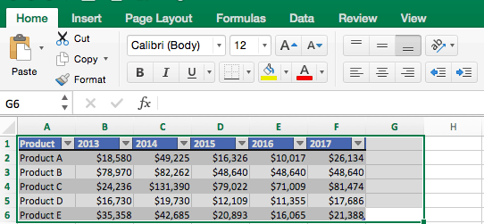
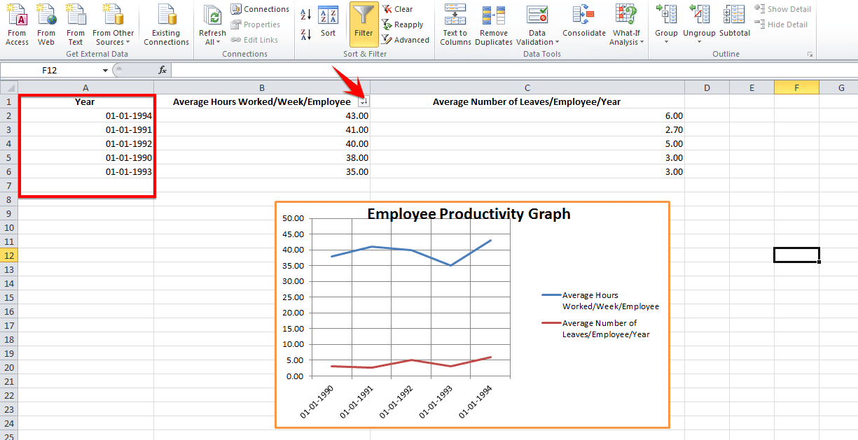
Refer to the below screenshot. Enter your data into excel. Here, we will use another method to create a trend chart in excel.
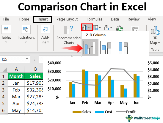
Alternatively, we can select the table and. This section will use a “double axis line graph and bar chart” to visualize the tabular data below. Use a scatter plot (xy chart) to show scientific xy data.
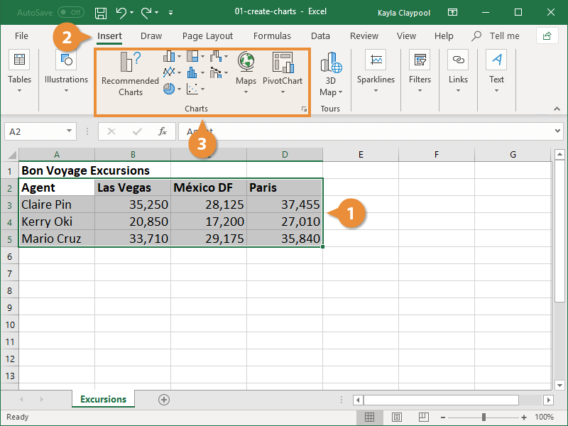
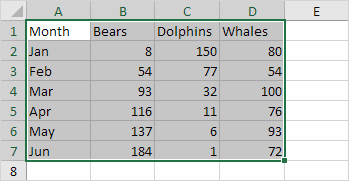
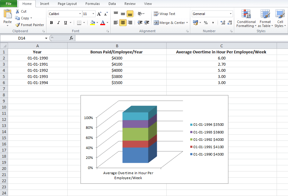
Now, you can change the color of the “base” columns to transparent or no fill. To get the desired chart you have to follow the following steps. First, click on a cell in the above table to select the entire table.
Follow the same steps as example #1. In the cell, f1 apply the formula for “average (b2:b31)”, where the function computes the average of 30 weeks. We want to add text inside the shapes, so let’s make them bigger.
Adjust the flowchart shape sizes. Using this formula we will create a trend chart. Learn the basics of excel charts to be able to quickly create graphs for your excel reports.
Excel 2013: Charts
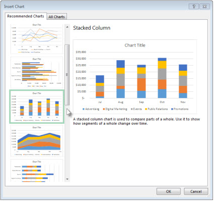
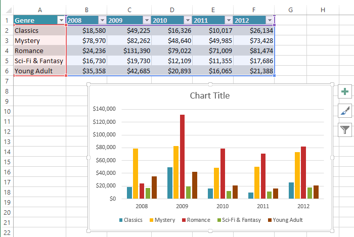
Create A Chart With Recommended Charts
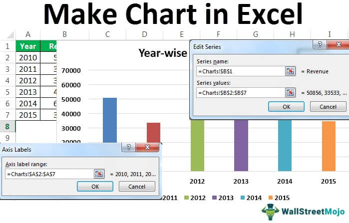
Add A Data Series To Your Chart

Create A Column Chart In Excel - Youtube
How To Make Charts And Graphs In Excel | Smartsheet
How To Create A Chart Or Graph In Excel?
How To Make Chart Or Graph In Excel? (step By Step Examples)
![How To Make A Chart Or Graph In Excel [With Video Tutorial]](https://lh6.googleusercontent.com/TI3l925CzYkbj73vLOAcGbLEiLyIiWd37ZYNi3FjmTC6EL7pBCd6AWYX3C0VBD-T-f0p9Px4nTzFotpRDK2US1ZYUNOZd88m1ksDXGXFFZuEtRhpMj_dFsCZSNpCYgpv0v_W26Odo0_c2de0Dvw_CQ)
How To Make A Chart Or Graph In Excel [with Video Tutorial]

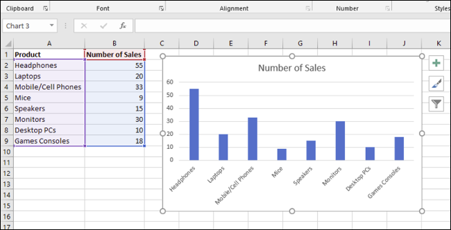
How To Create A Chart By Count Of Values In Excel?
How To Create Charts In Excel (in Easy Steps)
How To Make A Bar Chart In Microsoft Excel
How To Make A Graph In Excel: Step By Detailed Tutorial
How To Make A Graph In Excel: Step By Detailed Tutorial